![]()
This article showcases core functionalities of the package, and how to apply them in practice.
 Introduction
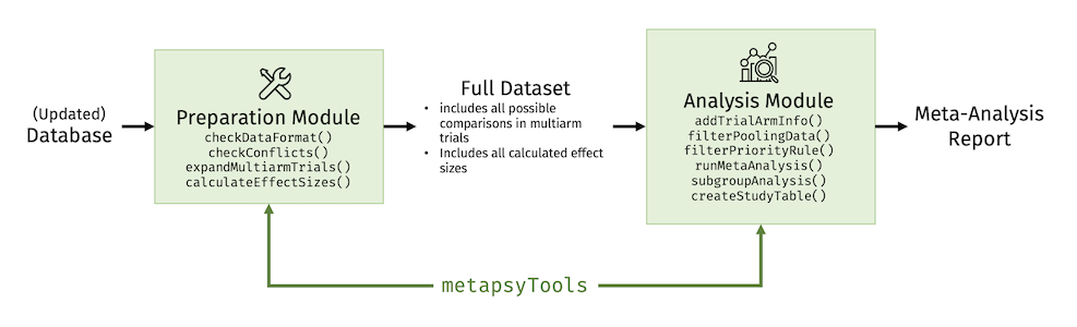
The metapsyTools package is part of the Metapsy project.
Functions included in the package can be used to run meta-analyses of
Metapsy databases, or
of databases that adhere to the same data
standard, “out of the box” using R.
The package also contains a set of tools that can be used to prepare meta-analytic data sets based on the Metapsy data standard, and to calculate effect sizes (Hedges’ and risk ratios, ).
The package consists of two modules:
- A module to check the data format and calculate effect sizes for all possible study comparisons (preparation module);
- A module to select relevant comparisons for a specific meta-analysis, calculate the results (including subgroup, meta-regression, and publication bias analyses), and generate tables (analysis module).
The idea is to use the two modules in different contexts. For example, the preparation module can be used every time the database is updated to gather all information, calculate effect sizes, and bring the data into a format suitable for further analyses.
Prepared data sets that follow the Metapsy data standard build the basis for the analysis module. Researchers simply have to filter out the comparisons that are relevant for the investigation, and can then use functions of the package to run a full meta-analysis, including sensitivity and subgroup analyses.
Important: The preparation module requires a
familiarity with the general structure of the database, as well as
intermediate-level knowledge of R and the metapsyTools
package itself, in order to diagnose (potential) issues. We advise that
the preparation step (i.e. checking the data format and calculating
effect sizes each time the database is updated) should be conducted by a
person with some proficiency in R & data wrangling. The analysis
module, on the other hand, should be usable by all researchers.
The companion package of metapsyTools is metapsyData. Using
metapsyData, meta-analytic databases can be automatically
downloaded into your R environment. Databases retrieved using
metapsyData can directly be analyzed using
metapsyTools.
If your goal is to analyze existing databases included in
Metapsy, only the analysis module in metapsyTools is
relevant to you. Click here
to navigate directly to the analysis module
section.
 The Preparation Module
The preparation module in metapsyTools allows to:
- check if the classes of variables in the imported data are set as required, using the checkDataFormat function.
- check for formatting conflicts which have to be resolved prior to any further steps, using the checkConflicts function.
- calculate Hedges’ and/or risk ratios () for each comparison, provided suitable data is available, and generate a data set ready for meta-analyses, using the calculateEffectSizes function.
Required Data Structure
For your own convenience, it is highly advised to strictly follow some data formatting rules prior to importing a data set for effect size calculations. If all of these rules are followed closely, it minimizes the risk of receiving error messages, producing conflicts, etc.
A detailed description of the preferred data structure can be found
in the Metapsy
documentation. The metapsyTools package also
includes a “toy” data set called depressionPsyCtr,
which has already been pre-formatted to follow the required data
format.
To use the data preparation module (i.e. calculate effect sizes), study design (I) and effect size data variables (II) must be included in the data set.
Study Design Variables (I)
-
study: The study name, formatted as “last name of the first author”, “year” (e.g."Smith, 2011"). -
condition_arm1: Condition in the first trial arm. The condition name is standardized to ensure comparability across trials (e.g.cbtfor all trial arms that employed cognitive-behavioral psychotherapy). -
condition_arm2: Condition in the second trial arm. The condition name is standardized to ensure comparability across trials (e.g.wlcfor all trial arms that employed a waitlist control group). -
multi_arm1: In multiarm trials, this variable provides a “specification” of the type of treatment used in the first arm. This variable is set toNA(missing) when the study was not a multiarm trial. For example, if a multiarm trial employed two types of CBT interventions, face-to-face and Internet-based, this variable would be set tof2fandInternet, respectively. -
multi_arm2: In multiarm trials, this variable provides a “specification” of the type of treatment used in the second arm. This variable is set toNA(missing) when the study was not a multiarm trial. For example, if a multiarm trial employed two types of control groups, waitlist and placebo, this variable would be set towlandplac, respectively. -
outcome_type: This variable encodes the type of outcome that builds the basis of the comparison, e.g."response","remission"or"deterioration". This variable is particularly relevant for dichotomous effect size data, because it indicates what the event counts refer to. The"msd"factor level is used for outcomes expressed in means and standard deviations. -
instrument: This variable describes the instrument through which the relevant outcome was measured. -
time: The measurement point at which the outcome was obtained (e.g.postorfollow-up). -
time_weeks: The measurement point at which the outcome was obtained, in weeks after randomization (set toNAif this information was not available). -
rating: This variable encodes if the reported outcome was self-reported ("self-report") or clinician-rated ("clinician").
Effect Size Data Variables (II)
Each Metapsy database also contains variables in which the (raw or
pre-calculated) effect size data is stored. In each row, one of the
following variable groups (a) to (d) are specified, depending on the
type of outcome data reported in the paper. The rest of the
variable groups will contain NA in that row.
When preparing the effect size data, it is very important that each
row only has data provided for one variable group (as defined below),
while the other variable groups are NA (i.e., have missing
values). Otherwise, the calculateEffectSizes
function that we use later will not know which type of effect size
should be calculated.
(a) Continuous Outcome Data
-
mean_arm1: Mean of the outcome in the first arm at the measured time point. -
mean_arm2: Mean of the outcome in the second arm at the measured time point. -
sd_arm1: Standard deviation of the outcome in the first arm at the measured time point. -
sd_arm2: Standard deviation of the outcome in the second arm at the measured time point. -
n_arm1: Sample size in the first trial arm. -
n_arm2: Sample size in the second trial arm.
(b) Change Score Data
-
mean_change_arm1: Mean score change between baseline and the measured time point in the first arm. -
mean_change_arm2: Mean score change between baseline and the measured time point in the second arm. -
sd_change_arm1: Standard deviation of the mean change in the first arm. -
sd_change_arm2: Standard deviation of the mean change in the second arm. -
n_change_arm1: Sample size in the first trial arm. -
n_change_arm2: Sample size in the second trial arm.
(c) Dichotomous Outcome Data (Response, Remission, Deterioration, …)
-
event_arm1: Number of events (responders, remission, deterioration cases) in the first trial arm. -
event_arm2: Number of events (responders, remission, deterioration cases) in the second trial arm. -
totaln_arm1: Sample size in the first trial arm. -
totaln_arm2: Sample size in the second trial arm.
(d) Pre-calculated Hedges’
-
precalc_g: The pre-calculated value of Hedges’ (small-sample bias corrected standardized mean difference; Hedges, 1981). -
precalc_g_se: Standard error of , viz. .
(d) Pre-calculated log-risk ratio
-
precalc_log_rr: The pre-calculated value of the log-risk ratio , comparing events in the first arm to events in the second arm. -
precalc_log_rr_se: The standard error of the log-risk ratio , comparing events in the first arm to events in the second arm.
Additional Considerations
Metapsy databases also contain additional variables. These are used, for example, to collect subject-specific information that is not relevant for all indications. Nevertheless, there are several formatting rules that all variables/columns follow:
- All variable names are in
snake_case. - Variable names start with a standard letter (
_is not allowed,.is only allowed formetapsyToolsvariables). - Variable names do not contain special characters (like @, ğ).
- Semicolons (
;) are not used; neither as variable names nor as cell content. - Character values contain no leading/trailing white spaces.
- Missing values are encoded using
NA.
Data Format & Conflict Check
Once the data set has been pre-structured correctly,
metapsyTools allows you to check the required variable
format and control for potential formatting conflicts.
If the formatting rules above are followed, none of the default
behavior of the preparation module has to be changed. At first, one can
run checkDataFormat. As an illustration, we will use the depressionPsyCtr
data frame, a pre-installed “toy” data set which is directly available
after installing metapsyTools.
# Load metapsyTools & dplyr
library(metapsyTools)
library(dplyr)

# Load preinstalled "toy" dataset
data("depressionPsyCtr")

# Check data format
depressionPsyCtr <- checkDataFormat(depressionPsyCtr)
# - [OK] Data set contains all variables in 'must.contain'.
# - [OK] 'study' has desired class character.
# - [OK] 'condition_arm1' has desired class character.
# [...]We see that the function has checked the required variables and their class. If divergent, the function will also try to convert the variable to the desired format.
Required variables for unique IDs: To function
properly, the metapsyTools functions must be able to
generate a unique ID for each comparison. By default, this is
achieved by combining information of the study,
condition_arm1, condition_arm2,
multi_arm1, multi_arm2,
outcome_type, instrument, time,
time_weeks, rating variables. These variables
are included by default in the must.contain argument in the
checkDataFormat function. If all required variables are
detected, an OK message is returned; as is the case in our
example.
We can also check the data for potential formatting issues, using the
checkConflicts function.
depressionPsyCtr <- checkConflicts(depressionPsyCtr)
# - [OK] No data format conflicts detected.In our case, no data format conflicts were detected. This is because all the data were pre-structured correctly. If data conflicts exist, the output looks similar to this:
# - [!] Data format conflicts detected!
# ID conflicts
# - check if variable(s) study create(s) unique assessment point IDs
# - check if specification uniquely identifies all trial arms in multiarm trials
# --------------------
# Abas, 2018
# Ammerman, 2013
# Andersson, 2005
# [...]
ID conflicts typically occur because the information in the variables
used to build the IDs (see box above) is not sufficient to create a
unique ID for each comparison. Studies with non-unique IDs are
subsequently printed out. The checkConflicts function also has an
argument called vars.for.id, which can be used define
(other or additional) columns to be used for ID generation. This can
sometimes help to create unique IDs.
As an illustration, we now define an extended variable list to be
used for our IDs in checkConflicts:
# Define extended ID list
# "target_group" is now also included
id.list <- c("study", "outcome_type",
             "instrument", "time", "time_weeks",
             "rating", "target_group")

# Use id.list as input for vars.for.id argument
checkConflicts(depressionPsyCtr,
               vars.for.id = id.list)
Effect Size Calculation
If the data set has been pre-formatted correctly, and all ID
conflicts were resolved, the calculateEffectSizes
function can be used to calculate effect sizes (Hedges’
or risk ratios,
)
for all comparisons in the database.
The calculateEffectSizes function uses the information
stored in the effect
size data variables to calculate
and/or
,
depending on what information is available. Therefore, it is very
important to make sure these variables are defined correctly before
running calculateEffectSizes.
The calculateEffectSizes function adds nine columns to
the data set, all of which start with a dot (.). They are
included so that meta-analysis functions in metapsyTools
can be applied “out of the box”.
-
.id: Unique identifier for a trial arm comparison/row. -
.g: Calculated effect size (Hedges’ ). -
.g_se: Standard error of Hedges’ . -
.log_rr: Calculated effect size (). -
.log_rr_se: Standard error of . -
.event_arm1: Number of events (e.g. responders) in the first trial arm. -
.event_arm2: Number of events (e.g. responders) in the second trial arm. -
.totaln_arm1: Total sample size in the first trial arm. -
.totaln_arm2: Total sample size in the second trial arm.
data <- calculateEffectSizes(depressionPsyCtr)Now, let us have a look at the calculated effect sizes ( and ) in a random slice of the data:
# Show rows 10 to 15, and variables "study", ".g", and ".log_rr"
data %>%
  slice(10:15) %>%
  select("study", ".g", ".log_rr")
# study .g .log_rr
# 10 Ahmadpanah, 2016 1.7788677 NA
# 11 Alexopoulos, 2016 0.2151835 -0.2436221
# 12 Alexopoulos, 2016 -0.2151835 0.2436221
# 13 Allart van Dam, 2003 -0.5696379 NA
# 14 Allart van Dam, 2003 0.5696379 NA
# 15 Ammerman, 2013 -0.9439887 NAWe see one important detail here. When dichotomous outcome data is
provided, the calculateEffectSizes
function automatically calculates both the log-risk ratio, and an
estimate of
.
Therefore, effects on remission, response, etc. are by default also
included in meta-analyses based on Hedges’
.
Please make sure to filter these effect sizes out if you do not want to
have them included in your meta-analysis. The filterPoolingData
function, which we will cover later, allows to do this.
Change Effect Size Sign
The change.sign argument in
calculateEffectSizes can be used to change the sign of one
or several calculated effect sizes (e.g. change the calculated effect
size from
=0.30
to
=-0.30,
or vice versa). This is illustrated below:
# Take a slice of the data for illustration
depressionPsyCtrSubset <- depressionPsyCtr %>% slice(10:15)

# Create a logical variable which, for each row,
# indicates if the sign of g should be changed
depressionPsyCtrSubset$sign_change <- c(TRUE, TRUE, TRUE,
                                        TRUE, TRUE, FALSE)

# Calculate effect sizes while defining the variable in
# our data in which the change sign information is stored
data.change.sign <- calculateEffectSizes(
                      depressionPsyCtrSubset,
                      change.sign = "sign_change")

# Show the relevant columns
data.change.sign %>%
  select(study, .g, .log_rr)
# study .g .log_rr
# 1 Ahmadpanah, 2016 -1.7788677 NA
# 2 Alexopoulos, 2016 0.2151835 -0.2436221
# 3 Alexopoulos, 2016 0.2151835 0.2436221
# 4 Allart van Dam, 2003 0.5696379 NA
# 5 Allart van Dam, 2003 -0.5696379 NA
# 6 Ammerman, 2013 -0.9439887 NAWe see that .g has now changed where ever
sign_change has been set to TRUE. We also see
that this does not affect the estimates of
.
Including Switched Arms
By default, Metapsy databases will only include all unique trial arm combinations, not all unique comparisons. To show when and why this difference matters, let us consider a small example.
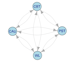
Imagine that we have data of a four-arm trial. Say that this trial included CBT, PST, CAU and a wait-list condition. While this trial provides 6 unique trial arm combinations1, the number of unique comparisons is higher: .
This is because the sign of the calculated effect size depends on which treatment serves as the reference. The effect of CBT vs. PST, for example, depends on which arm serves as the reference group (i.e. CBT vs. PST or PST vs. CBT). Depending on which arm is chosen (and assuming non-zero mean differences), the calculated effect size (e.g. Hedges’ ) value will either be negative (e.g. =-0.31) or positive (=0.31). We see this visualized in the graph below. There are now two directed arrows for each comparison (12 in total), and each arrow reads as “is compared to”:
To truly calculate all unique comparisons, we have to set
the include.switched.arms argument to TRUE
when running calculateEffectSizes.
data.switched.arms <- calculateEffectSizes(
                        depressionPsyCtr,
                        include.switched.arms = TRUE)
The resulting data frame data now includes all effect
sizes that can theoretically be calculated (assuming that all relevant
combinations were included in the original data).
Should I use include.switched.arms? It is not essential to calculate all possible arm comparisons. However, having all possible comparisons in your data set is convenient, because all required comparisons pertaining to a particular research question (e.g. “how effective is PST when CBT is the reference group?”) can directly be filtered out; there is typically no need for further data manipulation steps then.
The include.switched.arms argument can also be helpful
if you want to prepare network meta-analysis data
(which is subsequently analyzed using, e.g., the netmeta
package). However, this assumes that the data set already contains all
unique combinations in multi-arm trials (e.g. all 6
combinations in the four-arm study above, not just a selection).
This leads to our final data set which can be used with the analysis module, which will be described next.
 The Analysis Module
The analysis module in metapsyTools allows to run
different kinds of meta-analyses based on the final data set created by
the preparation module. It is designed to also be usable by researchers
who were not directly involved in the preparation step, and is less
demanding in terms of required background knowledge. Metapsy databases
included in metapsyData can
directly be used by the analysis module in
metapsyTools.
The analysis module allows, among other things, to:
- Filter data using strict rules, fuzzy string matching, or by
implementing prioritization rules (
filterPoolingDataandfilterPriorityRule)2. - Run conventional random-effects meta-analysis models, as well as
commonly reported sensitivity analyses (
runMetaAnalysis). - Correct effect estimates for potential publication bias or
small-study effects (
correctPublicationBias). - Run subgroup analyses based on the fitted model (
subgroupAnalysis) - Create study information tables (
createStudyTable).
Filtering Relevant Comparisons
The metapsyTools package contains functions which allow
to flexibly filter out comparisons that are relevant for a particular
meta-analysis.
The filterPoolingData
function is the main function for filtering. We simply have to provide
the final data set with calculated effect sizes (see preparation
module), as well as one or several filtering criteria pertaining to
our specific research question.
Say that we want to run a meta-analysis of all studies in which CBT was compared to wait-lists, with the BDI-I at post-test being the analyzed outcome. We can filter out the relevant comparisons like this:
# Load the pre-installed "depressionPsyCtr" dataset
load("depressionPsyCtr")
data <- depressionPsyCtr

# Filter relevant comparisons
data %>%
    filterPoolingData(
      condition_arm1 == "cbt",
      condition_arm2 == "wl",
      instrument == "bdi-1",
      time == "post") %>% nrow()
# [1] 7We see that
=7
comparisons fulfill these criteria. Note, however, that this will only
select comparisons for which condition_arm1 was
exactly defined as "cbt".
It is also possible to filter out all rows that simply
contain a specific search term (fuzzy
matching). For example, instead of "cbt", we might
want to filter out all studies that employed some type of “other”
therapy format. This can be achieved by using the Detect
function within filterPoolingData:
data %>%
  filterPoolingData(
    Detect(condition_arm1, "other")) %>%
  pull(condition_arm1)
# [1] "other psy" "other ctr" "other ctr" "other ctr" "other ctr" "other ctr"
# [7] "other ctr" "other ctr" "other psy"We can create even more complex filters. Say that we want to examine the effect, as measured by the BDI-I at post-test, of CBT, PST, and BAT compared to either CAU or wait-lists. We can visualize this with a graph again:
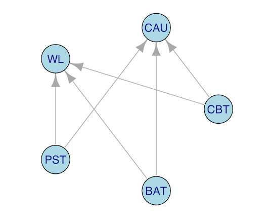
We can use the OR-Operator | within
filterPoolingData for such filter types. Again, we use the
Detect function to allow for fuzzy matching:
data %>%
  filterPoolingData(
    Detect(condition_arm1, "cbt|pst|bat"),
    Detect(condition_arm2, "cau|wl"),
    instrument == "bdi-1",
    time == "post") %>% nrow()
# [1] 11Lastly, one can also filter data according to a specified
priority rule, using the filterPriorityRule
function. This is particularly helpful to select instruments. Say, for
example, that we ordered certain instruments based on their known
reliability. Now, for each study, we only want to select the comparison
in which the most reliable instrument was used. It is possible that, for
some studies, all used instruments are relatively unreliable. However,
given our priority rule, we can still extract the comparison with a
relatively high reliability, and discard all the other
measurements within one study that are even less reliable.
Assume that our priority rule for the employed instrument is
"hdrs" (priority 1), "bdi-2" (priority 2),
"phq-9" (priority 3) and "bdi-1" (priority 4).
We can implement the rule like this:
data %>%

  # First, filter all other relevant characteristics
  filterPoolingData(
    Detect(condition_arm1, "cbt|pst|bat"),
    Detect(condition_arm2, "cau|wl"),
    time == "post") %>%

  # Now, implement the priority rule for the outcome instrument
  filterPriorityRule(
    instrument = c("hdrs", "bdi-2",
                   "phq-9", "bdi-1")) %>%

  # Show number of entries
  nrow()
# [1] 20Pooling Effects
After all relevant rows have been filtered out, we can start to pool
the effect sizes. The runMetaAnalysis
function serves as a wrapper for several commonly used meta-analytic
approaches, and, by default, applies them all at once to our data:
-
"overall". Runs a generic inverse-variance (random-effects) model. All included effect sizes are treated as independent. If raw event data is available in theevent_arm1,event_arm2,totaln_arm1,totaln_arm2columns (see Effect Size Calculation), the Mantel-Haenszel method (Greenland & Robins, 1985) is used to pool effects. Please note that assumptions of this model are violated whenever a study contributes more than one effect sizes (since these effect sizes are assumed to be correlated). In this case, results of the"combined"and"threelevel"/"threelevel.che"models should be reported instead. -
"combined". Aggregates all effect sizes within one study before calculating the overall effect. This ensures that all effect sizes are independent (i.e., unit-of-analysis error & double-counting is avoided). To combine the effects, one has to assume a correlation of effect sizes within studies, empirical estimates of which are typically not available. By default,runMetaAnalysisassumes that =0.6. -
"lowest.highest". Runs a meta-analysis, but with only (i) the lowest and (ii) highest effect size within each study included. -
"outlier". Runs a meta-analysis without statistical outliers (i.e. effect sizes for which the confidence interval does not overlap with the confidence interval of the overall effect). -
"influence". Runs a meta-analysis without influential cases, as defined using the influence diagnostics in Viechtbauer & Cheung (2010). See also theInfluenceAnalysisfunction indmetar, and Harrer et al. (2022, chap. 5.4.2). -
"rob". Runs a meta-analysis with only low-RoB studies included. By default, only studies with a value> 2in therobvariable are considered for this analysis. -
"threelevel". Runs a multilevel (three-level) meta-analysis model, with effect sizes nested in studies (Harrer et al., 2022, chap. 10). -
"threelevel.che". Runs a multilevel (three-level) “correlated and hierarchical effects” (CHE) meta-analysis model. In this model, effect sizes are nested in studies, and effects within studies are assumed to be correlated (Pustejovsky & Tipton, 2022; by default, it is assumed that =0.6). This will typically be a plausible modeling assumption in most real-world use cases. In most scenarios, the"threelevel.che"model can be seen as a better (and therefore preferable) approximation of the data structure at hand, compared to the simpler"threelevel"model.
To illustrate how the function works, we first select a subset of our
“toy” depressionPsyCtr data.
# Only select data comparing CBT to waitlists and CAU
depressionPsyCtr %>%
  filterPoolingData(
    condition_arm1 == "cbt",
    Detect(condition_arm2, "wl|cau")
  ) -> ma.data
Then, we plug the resulting ma.data data set into the
runMetaAnalysis function:
res <- runMetaAnalysis(ma.data)# - Running meta-analyses...
# - [OK] Using Hedges' g as effect size metric...
# - [OK] Calculating overall effect size... DONE
# - [OK] Calculating effect size using only lowest effect... DONE
# - [OK] Calculating effect size using only highest effect... DONE
# - [OK] Calculating effect size using combined effects (rho=0.6; arm-wise)... DONE
# - [OK] Calculating effect size with outliers removed... DONE
# - [OK] Calculating effect size with influential cases removed... DONE
# - [OK] Calculating effect size using only low RoB information... DONE
# - [OK] Calculating effect size using three-level MA model... DONE
# - [OK] Robust variance estimation (RVE) used for three-level MA model... DONE
# - [OK] Calculating effect size using three-level CHE model (rho=0.6)... DONE
# - [OK] Robust variance estimation (RVE) used for three-level CHE model... DONE
# - [OK] Done!As we can see, while running, the runMetaAnalysis
function provides us with a few messages that allow to trace if all
models have been fitted successfully. When there are problems during the
calculation, the runMetaAnalysis function will print a
warning.
# This tells the function to only consider studies with a rob score
# above 4 in the "low risk of bias" sensitivity analysis
runMetaAnalysis(ma.data, low.rob.filter = "rob > 4")
# [...]
# - [!] No low risk of bias studies detected! Switching to 'general'... DONE
# [...]We can inspect the results by calling the created res
object in the console.
res# Model results ------------------------------------------------
# Model k g g.ci p i2 i2.ci prediction.ci nnt
# Overall 26 -0.57 [-0.85; -0.28] <0.001 76.4 [65.65; 83.76] [-1.57; 0.43] 5.22
# Combined 17 -0.54 [-0.89; -0.18] 0.005 77.1 [63.64; 85.57] [-1.64; 0.57] 5.56
# One ES/study (lowest) 14 -0.57 [-1; -0.13] 0.015 79.8 [66.82; 87.65] [-1.78; 0.64] 5.22
# One ES/study (highest) 14 -0.47 [-0.84; -0.11] 0.015 73.9 [55.75; 84.62] [-1.45; 0.5] 6.41
# Outliers removed 23 -0.46 [-0.63; -0.29] <0.001 61.6 [39.55; 75.55] [-1.11; 0.19] 6.64
# Influence Analysis 24 -0.43 [-0.6; -0.27] <0.001 63.9 [44.18; 76.66] [-1.08; 0.22] 7.08
# Only rob > 2 13 -0.34 [-0.58; -0.11] 0.008 73.4 [53.91; 84.71] [-1.1; 0.41] 9.12
# Three-Level Model 26 -0.61 [-1.05; -0.17] 0.011 92.1 - [-2.17; 0.96] 4.81
# Three-Level Model (CHE) 26 -0.55 [-0.92; -0.18] 0.007 88 - [-1.8; 0.7] 5.42
#
# Variance components (three-level model) ----------------------
# Source tau2 i2
# Between Studies 0.536 92.1
# Within Studies 0 0
# Total 0.536 92.1
#
# Variance components (three-level CHE model) ------------------
# Source tau2 i2
# Between Studies 0.336 87.2
# Within Studies 0.003 0.8
# Total 0.339 88 By default, an HTML table should pop up along with
the console output. These pre-formatted HTML results tables can easily
be transferred to, for example, MS Word using copy and paste. To disable
this feature, we have to specify html=FALSE inside the
function call.
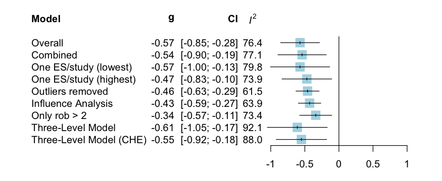
Using the summary method, details of the analysis
settings can be printed. This function also returns recommended
citations for the applied methods and/or packages. Furthermore, it
creates a summary forest plot in which all pooled
effects are displayed.
summary(res)## Analysis settings ----------------------------------------------------------
##
## ✓ [Overall] Random effects model assumed.
## ✓ [Overall] Heterogeneity variance (tau2) calculated using restricted maximum-likelihood estimator.
## ✓ [Overall] Test statistic and CI of the pooled effect calculated using the Knapp-Hartung adjustment.
## ✓ [Outliers removed] ES removed as outliers if the CI did not overlap with pooled effect CI.
## ✓ [Influence Analysis] Influential cases determined using diagnostics of Viechtbauer and Cheung (2010).
## [...]
##
##
## Cite the following packages/methods: ---------------------------------------
##
## - {meta}: Balduzzi S, Rücker G, Schwarzer G (2019),
## How to perform a meta-analysis with R: a practical tutorial,
## Evidence-Based Mental Health; 22: 153-160.
## - {metafor}: Viechtbauer, W. (2010). Conducting meta-analyses in R
## with the metafor package. Journal of Statistical Software, 36(3), 1-48.
## https://doi.org/10.18637/jss.v036.i03.
## [...]
Additional Arguments
The runMetaAnalysis function allows to tweak many, many
details of the specific meta-analysis models (run
?runMetaAnalysis to see the entire documentation). The most
important arguments one may want to specify are:
-
es.measure. By default, the function conducts analyses using the Hedges’ values stored in the data set. To conduct analyses using dichotomous outcome data (i.e. response, remission, etc.), one has to set this argument to"RR"(for risk ratios),"EER"(for intervention group response rates), or"CER"(for control group response rates). -
es.type. By default, analyses are conducted using the"precalculated"effect sizes stored in the prepared data set. For risk ratios, one can alternatively set this argument to"raw", which means that the “raw” event counts are used for computations (instead of the pre-calculated log-risk ratio and its standard error). This is typically preferable, but may not be possible if this information could not be extracted from all primary studies. -
method.tau. This argument controls the method to be used for estimating the between-study heterogeneity variance . The default is"REML"(restricted maximum likelihood), but other options such as the DerSimonian-Laird estimator ("DL") are also available (see therunMetaAnalysisfunction documentation for more details). Note that three-level meta-analysis models can only be fitted using (restricted) maximum likelihood. -
nntCer. TherunMetaAnalysisfunction uses the method by Furukawa and Leucht (2011) to calculate the Number Needed to Treat (NNT) for each pooled effect size. This method needs an estimate of the control group event rate (CER). By default,nntCer = 0.2is used, but you can set this to another value if desired. -
rho.within.study. To combine effect sizes on a study level before pooling ("combined"model), one has to assume a within-study correlation of effects. By default,rho.within.study = 0.6is assumed, but this value can and should be changed based on better approximations. This value also controls the assumed within-study correlation in the multilevel CHE model ("threelevel.che"). -
low.rob.filter. By default, the function uses all comparisons for which the risk of bias rating in therobvariable has a value greater2(low.rob.filter = "rob > 2"). If your risk of bias rating is in another variable, or if another threshold should be used, you can change this argument accordingly.
Here is an example of a runMetaAnalysis call with
non-default settings:
runMetaAnalysis(ma.data,
                es.measure = "RR",
                es.type = "raw",
                method.tau = "DL",
                nntCer = 0.4,
                rho.within.study = 0.8)
Also note that for the "combined" model, by default,
effect sizes of multi-arm trials will be aggregated on an
arms level. If, for example, a study
included a CBT, Internet-based CBT, and wait-list arm (where wait-list
is the reference condition), two separate aggregated effects will be
calculated: one for CBT vs. wait-list, and one for Internet-based CBT
vs. wait-list.
From a statistical perspective, it is typically preferable to aggregate on a study level instead3 (in our example, this would lead to one aggregated effect for CBT/Internet-based CBT combined vs. wait-list), although the aggregated effect sizes may then be more difficult to interpret from a clinical perspective.
To combine effect sizes on a study level instead, we can set the
which.combine argument to "studies".
runMetaAnalysis(ma.data, which.combine = "studies")Confidence Intervals for Three-Level Model and Values
Please note that, by default, no confidence intervals are printed for
the
value of the "threelevel" and "threelevel.che"
model (the same is also the case for the
value, the equivalent of
in limit meta-analyses; see Publication
Bias section)4. This is because there are two
heterogeneity variances in three-level models: the “conventional”
between-study heterogeneity variance
and the heterogeneity variance within studies,
.
This means that there are also two
values, one within studies, and one for the between-study heterogeneity.
Established closed-form or iterative solutions (such as the
-Profile
method; Viechtbauer, 2007) are not
directly applicable here, which means that confidence intervals cannot
be calculated that easily.
In metapsyTools, one can resort to the
parametric bootstrap (van den Noortgate & Onghena,
2005)
to obtain approximate confidence intervals around the
and
values. Bootstrapping is performed when the i2.ci.boot
argument is set to TRUE. By default,
=5000
bootstrap samples are drawn, which should be seen as the absolute lower
limit; more replications are preferable and can be specified via the
nsim.boot argument.
Please note that the bootstrapping is computationally expensive, which means that it can take up to an hour and longer until final results are obtained. During the bootstrapping procedure, the function prints a progress update so that users get an indication of how long the function (still) has to run.
res.boot <- runMetaAnalysis(ma.data,
                            i2.ci.boot = TRUE,
                            nsim.boot = 500)
res.boot
# 1% completed | 2% completed | 3% completed ...Confidence intervals around and the will then be printed out along with the usual results.
# [...]
# Variance components (three-level model) ----------------------
# Source           tau2 tau2.ci           i2 i2.ci
# Between Studies 0.536 [0.178; 1.092]  92.1 [74.29; 95.72]
# Within Studies  0     [0; 0.055]       0   [0; 10.43]
# Total           0.536 [0.182; 1.107]  92.1 [79.83; 96.01]
#
# Variance components (three-level CHE model) ------------------
# Source           tau2 tau2.ci           i2 i2.ci
# Between Studies 0.336 [0.068; 0.667]  87.2 [56.65; 92.9]
# Within Studies  0.003 [0; 0.03]        0.8 [0; 10.31]
# Total           0.339 [0.079; 0.681]  88   [63.17; 93.67]
When runMetaAnalysis was run with
i2.ci.boot set to TRUE, the
(or, more correctly,
)
value of the limit meta-analysis will also be
calculated using parametric bootstrapping, provided that
correctPublicationBias is called afterwards (see publication
bias section).
Complex Variance-Covariance Approximation
The vcov argument in
runMetaAnalysiscontrols if the effect size dependencies
within the data should be approximated using a "simple"
(default) or more "complex" (but potentially more accurate)
method. This argument is only relevant for the "combined"
and "threelevel.che" models. The default “simple” method
constructs variance-covariance matrices
for each study using a constant sampling correlation
(defined by rho.within.study), which is identical across
all studies, outcomes, and time points. This simplifying assumption is
part of the formulation of the CHE model originally provided by
Pustejovsky and Tipton (2022).
Naturally, employing a common value of
across all studies may not be reasonable in some analyses, and other
information may be available to better approximate the effect size
dependencies in the collected data. Setting vcov to
"complex" allows to assume that correlations between effect
sizes may differ conditional on the type of dependency. This means that
the variance-covariance matrix
of some study
is approximated by an unstructured matrix with varying
.
Put simply, this method allows to account for the fact that there can be various types of effect size dependencies (e.g. effect sizes are dependent because different instruments were used on the same sample; or they are dependent because effects of two different intervention groups were compared to the same control group in a multi-arm trial, and so on) and that, therefore, the magnitude of the correlation also differs.
Setting vcov = "complex" allows to additionally
incorporate assumed correlations specific to multiple testing over time
(e.g. correlations between effects at post-test and long-term
follow-up). The value provided in phi.within.study
represents the (auto-)correlation coefficient
,
which serves as a rough estimate of the re-test correlation after 1
week. This allows to model the gradual decrease in correlation between
measurements over time.
Furthermore, it is possible to calculate a correlation coefficient
for multi-arm trials, which is directly proportional to
the size of each individual trial arm. When all trial arms have the same
size, meaning that each arm’s weight
is identical,
is known to be 0.5. Multiarm weights
(and thus
)
can be derived if the w1.var and w2.var
variables, containing the sample size of each study arm, are
available.
Using the complex approximation method increases the risk that at least one studies’ matrix is not positive definite. In this case, the function automatically switches back to the constant sampling correlation approximation.
If the supplied data set format strictly follows the Metapsy
data standard, it is possible to set vcov to
"complex" without any further preparation steps. The
function will then inform us if the complex variance-covariance
approximation was not possible, meaning that the function automatically
reverted to the standard "simple" approach.
runMetaAnalysis(ma.data,
                vcov = "complex")
If you want to use the complex variance-covariance matrix approximation feature, it is advised to make sure that the data set contains the following columns:
"n_arm1"and"n_arm2": sample sizes in the two compared groups."time_weeks": post-randomization time point at which the measurement was made (in weeks).
For a correctly preformatted dataset, users are referred to the depressionPsyCtr
“toy” dataset.
Internal Objects
It is important to note that runMetaAnalysis is a
wrapper function. It provides a common interface to run
several meta-analysis models, while the models themselves are fitted
internally by other packages. In particular, we use functionality
provided by the meta (Balduzzi, Rücker & Schwarzer, 2019), metafor
(Viechtbauer, 2010),
and dmetar
(Harrer, Cuijpers, Furukawa & Ebert, 2019) packages.
When returning the results, runMetaAnalysis saves all
fitted models inside the returned object. Depending on their type, these
internal meta-analysis models work just like regular
meta or metafor models, which means that all
functionality developed for them is also available.
It is also possible to directly extract each calculated model from
the runMetaAnalysis results object. Each of these models
are identical to the ones one would receive by running metagen,
metabin,
or rma.mv
directly.
res$model.overall         # "overall" model (metagen/metabin)
res$model.combined        # "combined" model (metagen/metabin)
res$model.lowest          # lowest effect size/study only model (metagen/metabin)
res$model.highest         # highest effect size/study only model (metagen/metabin)
res$model.outliers        # outliers removed model (metagen/metabin)
res$model.influence       # influential cases removed model (metagen/metabin)
res$model.rob             # low RoB model (metagen/metabin)
res$model.threelevel      # three-level model
res$model.threelevel.che  # three-level CHE model
This means that any kind of operation available for
metagen or rma models is also
available for the models created by
runMetaAnalysis. For example, we can generate a
funnel plot for our “overall” model like this:
library(meta)

# model.overall is a "meta" model, so we can directly
# Apply the funnel function included in meta
funnel(res$model.overall,
       studlab = TRUE,
       contour = c(0.9, 0.95, 0.99),
       col.contour = c("darkgreen", "green", "lightgreen"))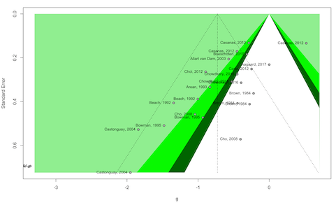
This feature can also be used to run, for example, Egger’s
regression test, using functions already included in
meta and dmetar:
# Egger's regression test applied to the "overall" model:
library(dmetar)
eggers.test(res$model.overall)
# Eggers' test of the intercept
# =============================
#
# intercept 95% CI t p
# -2.814 -3.97 - -1.66 -4.785 7.17608e-05
#
# Eggers' test indicates the presence of funnel plot asymmetry. For an overview of all available functionality, you can consult the specific documentation entry for each meta-analysis model type:
"overall","combined","lowest","highest","outliers","influence","rob": run?metagenin the console (if effect size is , or if effect size is andes.typeis"precalculated"); otherwise, run?metabin."threelevel"and"threelevel.che": run?rma.mvin the console. The methods section in this documentation entry is particularly relevant, since it shows functions that can be applied to this model type (so-called S3 methods).
Forest Plots
It is also possible to generate forest plots of all
the calculated models. We only have to plug the results object into
plot, and specify the name of the model for which the
forest plot should be retrieved:
plot(res, "overall")        # Overall model (ES assumed independent)
plot(res, "combined")       # ES combined within studies before pooling
plot(res, "lowest.highest") # Lowest and highest ES removed (creates 2 plots)
plot(res, "outliers")       # Outliers-removed model
plot(res, "influence")      # Influential cases-removed model
plot(res, "threelevel")     # Three-level model
plot(res, "threelevel.che") # Three-level CHE model
This is what the "overall" model forest plot looks like,
for example:
plot(res, "overall")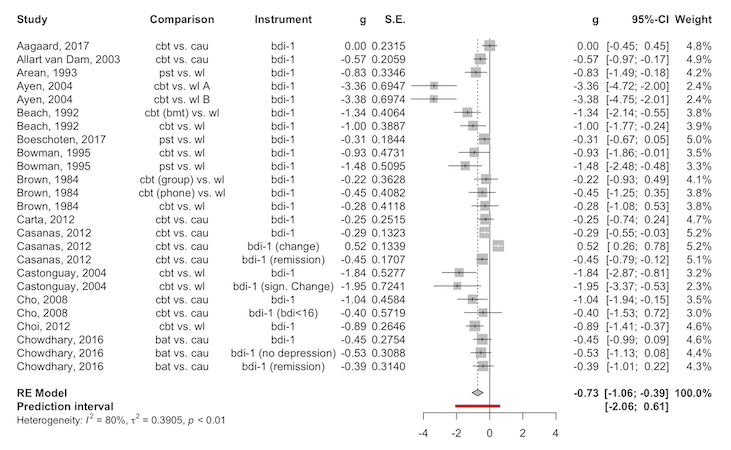
Note that the plot function is simply a wrapper for the
forest.meta function in the meta package.
Therefore, all the advanced styling
options are also available using extra arguments.
plot(res, "overall",
     col.predict = "lightgreen",
     col.square = "gray",
     fontfamily = "Palatino")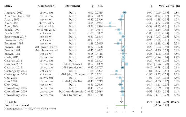
It is also possible to generate Baujat and Leave-One-Out Plots (not displayed here).
Replacement Functions
Once a model has been fitted using runMetaAnalysis,
replacement functions are defined for each function
argument. This allows to quickly tweak one or more analysis settings,
which are implemented once the rerun function is
called.
If, for example, we want to check the results using a different estimator of , and a different CER to calculate the number needed to treat, leaving all other settings the same, we can run:
method.tau(res) <- "PM"
nntCer(res) <- 0.7
Then, we have to call the rerun function:
rerun(res)A list of all available setting replacement functions is provided here. Replacement functions may be particularly helpful for sensitivity analyses.
Publication Bias
It is also possible to correct effect size estimates for potential
publication bias and/or small-study effects using the correctPublicationBias
function. This will apply three correction methods at the same time,
providing a range of (more or less) plausible corrected values. Using
the which.run argument, we can apply these methods to a
specific model we fitted previously.5 Here, we select the "combined"
analysis.
correctPublicationBias(res, which.run = "combined")# [...]
# Publication bias correction ('combined' model) -----------------------
# Model k g g.ci p i2 i2.ci prediction.ci nnt
# Trim-and-fill method 24 -0.16 [-0.62; 0.31] 0.490 85.4 [79.41; 89.61] [-2.16; 1.85] 24.4
# Limit meta-analysis 17 0.1 [-0.32; 0.52] 0.649 95.1 - [-1.05; 1.25] 35.4
# Selection model 17 -0.87 [-1.38; -0.36] <0.001 85.7 [64.72; 94.57] [-1.98; 0.24] 6.38
# [...]The reason why three publication bias methods are applied at the same time is because all publication bias methods are based on (to some extent) untestable assumptions, and these assumption differ between methods:
The trim-and-fill method is included mostly as a “legacy” method, given its popularity in the last decades. This method is also frequently requested by reviewers. However, it has been found that this method does not perform well as a way to correct for publication bias, especially when the between-study heterogeneity is high. The trim-and-fill method assumes that publication bias results in funnel plot asymmetry, and provides an algorithm that imputes studies so that this asymmetry is removed, after which the results are re-estimated.
The limit meta-analysis method assumes that publication bias manifests itself in so-called small-study effects (i.e., it assumes that small studies with high standard errors are more likely to be affected by publication bias). It calculates the expected (“shrunken”) pooled effect as the standard error goes to zero, while accounting for between-study heterogeneity. Importantly, this methods controls for small-study effects only, which can be associated with publication bias, but does not have to.
Lastly, a step function selection model is calculated, which allows to account for the possibility that results are more or less likely to get published depending on their value. By default, the
selmodelStepsargument is set to 0.05, which means that we assume that results with <0.1 are more likely to get published. It is also possible to define more than one selection threshold, e.g. by settingselmodelStepstoc(0.025, 0.05).
For further details, see Harrer, Cuijpers, Furukawa & Ebert (2022, chap. 9.3).
The correctPublicationBias function also allows to
provide additional arguments that will be applied if they match the ones
defined in the trimfill
and limitmeta
functions in meta and metasens (Schwarzer,
Carpenter & Rücker, 2022),
respectively. You can find an example below:
correctPublicationBias(

              res, which.run = "combined",

              # Use the R-type estimator to trim & fill
              type = "R",

              # Use a random-effects model without bias parameter
              # to shrink effects in the limit meta-analysis
              method.adjust = "mulim")
Subgroup Analysis
The subgroupAnalysis function can be used to perform
subgroup analyses. Every column included in the data set initially
supplied to runMetaAnalysis can be used as a subgroup
variable.
For example, we might want to check if effects differ by country
(country) or intervention type
(condition_arm1):
sg <- subgroupAnalysis(res, country, condition_arm2)
sg
# Subgroup analysis results ----------------------
# variable group n.comp g g.ci i2 i2.ci nnt p
# country 3 13 -0.61 [-1.3; 0.07] 81.5 [69.5; 88.8] 4.80 0.666
# . 1 13 -0.76 [-0.93; -0.58] 0 [0; 56.6] 3.74 .
# condition_arm2 cau 12 -0.32 [-0.54; -0.09] 71.9 [49.6; 84.3] 9.90 0.025
# . wl 14 -0.96 [-1.54; -0.38] 70.6 [49.4; 83] 2.88 . By default, an HTML table should also pop up. The p
column to the right represents the significance of the overall subgroup
effect (there is, for example, no significant moderator effect of
country).
It is also possible to conduct subgroup analyses using another model,
say, the three-level model. We only have to specify
.which.run:
sg <- subgroupAnalysis(res,
                       country, condition_arm2,
                       .which.run = "threelevel")
When the number of studies in subgroups are small, it is sensible to
use a common estimate of the between-study
heterogeneity variance
(in lieu of subgroup-specific estimates). This can be done by setting
the .tau.common argument to TRUE in the
function:
sg <- subgroupAnalysis(res,
                       country, condition_arm2,
                       .which.run = "combined",
                       .tau.common = TRUE)
Meta-Regression
Since the runMetaAnalysis function saves all fitted
models internally, it is also possible to extract each of them
individually to do further computations. Say, for example, that we want
to perform multiple meta-regression using our threelevel
model. We want to use the risk of bias rating, as well as the scaled
study year as predictors. This can be achieved by extracting the model
to be analyzed using the $ operator, and then using
metaRegression to fit the model.
metaRegression(res$model.threelevel,
               ~ scale(as.numeric(rob)) + scale(year))
# Multivariate Meta-Analysis Model (k = 26; method: REML)
#
# Variance Components:
#
# estim sqrt nlvls fixed factor
# sigma^2.1 0.3821 0.6181 14 no study
# sigma^2.2 0.0000 0.0000 26 no study/es.id
#
# Test for Residual Heterogeneity:
# QE(df = 23) = 64.6042, p-val < .0001
#
# Test of Moderators (coefficients 2:3):
# F(df1 = 2, df2 = 23) = 3.0051, p-val = 0.0693
#
# Model Results:
#
# estimate se tval df pval ci.lb ci.ub
# intrcpt -0.6999 0.1923 -3.6394 23 0.0014 -1.0978 -0.3021 **
# scale(as.numeric(rob)) 0.5538 0.2364 2.3428 23 0.0282 0.0648 1.0428 *
# scale(year) -0.2656 0.2827 -0.9395 23 0.3572 -0.8503 0.3192
#
# ---
# Signif. codes: 0 ‘***’ 0.001 ‘**’ 0.01 ‘*’ 0.05 ‘.’ 0.1 ‘ ’ 1Please note that, to be available in metaRegression, it
is necessary that the moderator variable(s) are already included in the
data set that we originally used to call
runMetaAnalysis.
Risk of Bias
Databases formatted using the Metapsy data
standard will typically also contain risk of bias ratings for each
included study. The metapsyTools package also includes some
functionality to include and display this information during the
analysis.
To include risk of bias data, the data.rob argument has
to be specified when running runMetaAnalysis. In
particular, we need to first create and then provide a list element with
all the specifications. A documentation on how to specify this list
element is provided here.
# Define ROB data to be added to the models
robData = list(
  domains = c("sg", "ac", "ba", "itt"),
  domain.names = c("Sequence Generation",
                   "Allocation Concealment",
                   "Blinding of Assessors",
                   "ITT Analyses"),
  categories = c("0", "1", "sr"),
  symbols = c("-", "+", "s"),
  colors = c("red", "green", "yellow"))

# Re-run model with appended ROB data
res = runMetaAnalysis(ma.data, rob.data = robData)
Once this is set up, we can use the runMetaAnalysis
object to easily produce forest plots that include risk of bias
information.
plot(res, "threelevel.che",
     leftcols = c("study", "instrument"),
     leftlabs = c("Study", "Instrument"),
     smlab = "", fontfamily = "Tahoma",
     col.square = "lavender", col.predict = "black")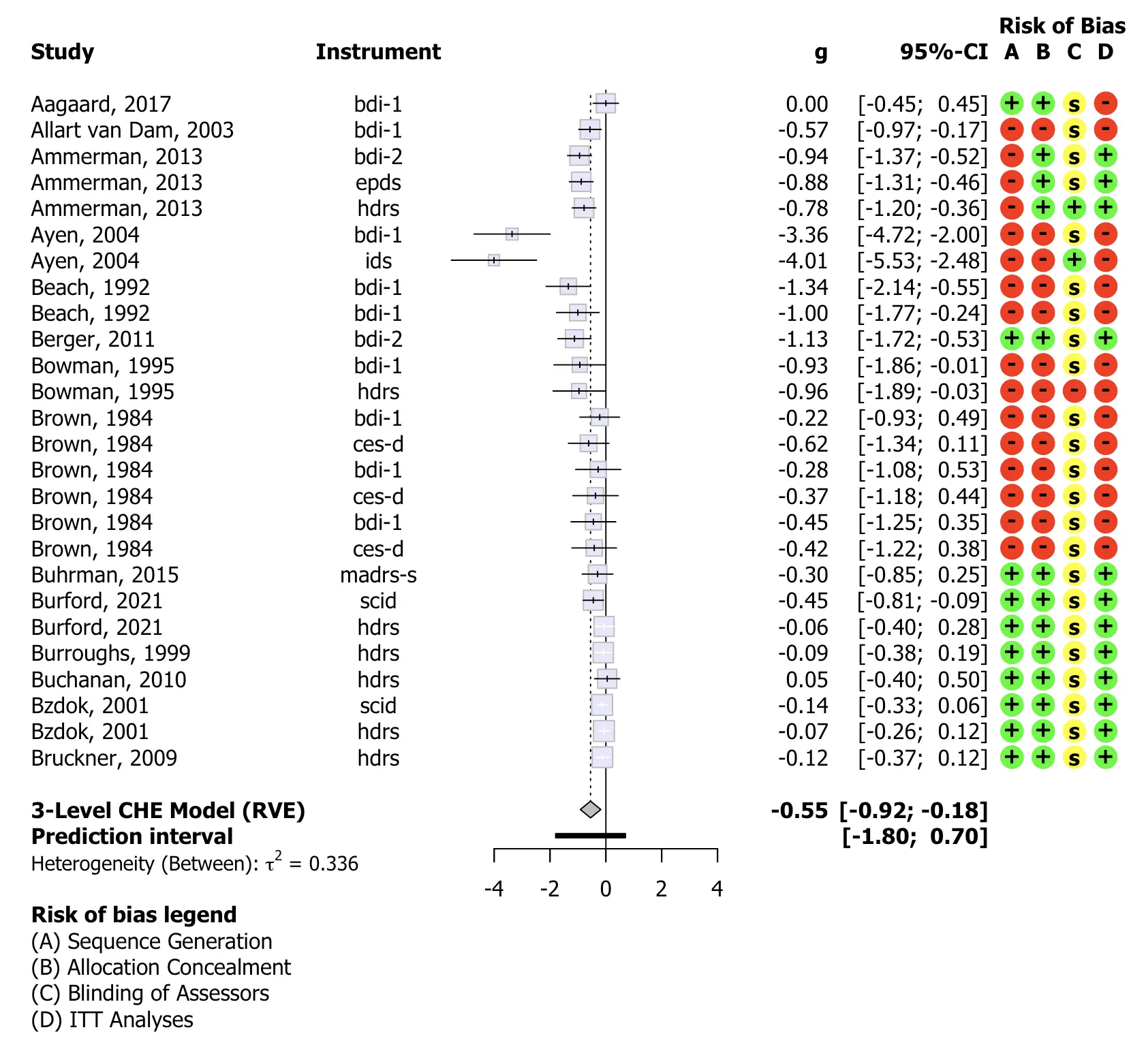
It is also possible to create a summary risk of bias plot, using the
createRobSummary function.
createRobSummary(res,
                 name.low = "1",
                 name.high = "0",
                 name.unclear = "sr")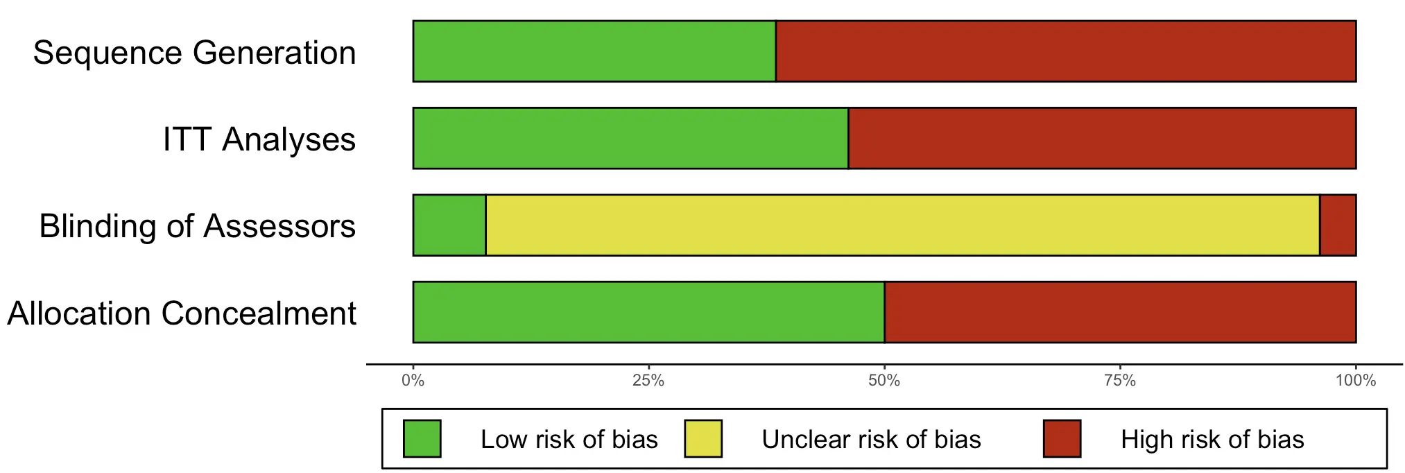
 Study Tables
The createStudyTable function allows to create an
overview table for the included studies/comparisons. One only has to
supply the filtered data set first, and then the names of the desired
variables in the order in which they should appear in the table. It is
also possible to rename factor labels directly in the function,
determine how far values should be rounded, and if variable names should
be changed:
createStudyTable(

  # Dataset. Alternatively, a runMetaAnalysis
  # object can also be used.
  ma.data,

  ## Columns --------------------------------------
  # Simply add columns in the order in which
  # they should appear in the table
  study, age_group, mean_age, percent_women,

  # You can directly recode values within a variable
  condition_arm1 = c("CBT" = "cbt"),
  multi_arm1,
  condition_arm2 = c("Wait-List" = "wl",
                     "Care-As-Usual" = "cau"),
  n_arm1, n_arm2,
  country = c("Europe" = "3", "USA" = "1"),
  sg, ac, itt,


  ## Specifications -------------------------------
  # .round.by.digits controls the number of rounded digits for
  # specified columns
  .round.by.digits = list(mean_age = 0,
                          n_arm1 = 0,
                          n_arm2 = 0),

  # .column.names allows to rename columns
  .column.names = list(age_group = "age group",
                       mean_age = "mean age",
                       percent_women = "% female",
                       condition_arm1 = "Intervention",
                       condition_arm2 = "Control",
                       n_arm1 = "N (IG)",
                       n_arm2 = "N (CG)",
                       multi_arm1 = "Specification"))
By default, createStudyTable also returns an HTML table
that one can copy and paste into MS Word.
Still have questions? This vignette only provides a
superficial overview of metapsyTools’ functionality. Every
function also comes with a detailed documentation, which you may consult
to learn more about available options and covered use cases. Please note
that metapsyTools is still under active development, which
means that errors or other problems may still occur under some
circumstances. To report an issue or ask for help, you can contact
Mathias (mathias.harrer@tum.de).